Valuation multiples how high is too high

Deciding whether a trading multiple is too high or too low can be a daunting task. For example, you may wonder if a stock trading at 20x P/E is overvalued. But when does a multiple become too high? This article offers a practical framework that can help you decide how high is too high.

 

What is a valuation multiple

Any multiple is simply the ratio between a valuation metric and a driver of value:

 

 

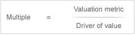
In the P/E multiple, the valuation metric (numerator) is the price per share, and the value driver is the EPS (denominator).

 

 

 

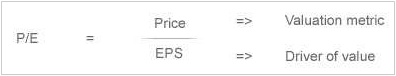
The fundamental logic of a multiple is that the value driver  (the denominator) must drive the value metric  (the numerator). In other words, there must be a proportional relationship between the two inputs: as the value driver increases, so does the value metric. In the P/E multiple case, most investors are likely to agree that an increase in net income will increase the firm’s equity value (everything else being equal). Therefore, if the EPS increases (denominator), so will the stock price (numerator)

 

P/E Multiple Valuation

To examine the relationship between stock price and EPS more precisely, we can express the stock price as the present value of a perpetuity of dividends:

 

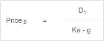
Where D1 is the dividend per share paid at time 1, Ke  is the cost of equity and g is the long- term growth rate of the dividend per share. If we now divide both sides by EPS, we obtain the formula for the P/E multiple:

 

 

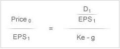
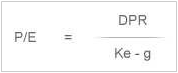
The numerator (D1 / EPS1) is the dividend payout ratio (DPR), which expresses the % of earnings paid out as dividends. Therefore, we can simplify the formula as follows:

 

 

Conclusion

The forward P/E multiple is determined by three drivers

 

1. Payout ratio
2. Cost of equity
3. Growth rate in profits

 

Notice that the value of the three drivers needs to stay constant over a long period of time for the P/E formula to hold.

 

Practical application – reverse engineering the multiple

Any observed P/E value can be reverse-engineered to analyze the implied assumptions about its drivers.

 

Example 1 – Implied Perpetuity Growth Rate

We analyze a mature business with a dividend policy of around 80% payout and an estimated cost of equity of 8%. The stock is trading at 10x P/E. What is its implied long-term growth rate? The answer is: 0%. Is that growth realistic? Or is it too low? Assuming a growth rate of 3%, the stock should be trading at a P/E of 16x. Is this stock a buy?

 

Example 2 – The implied payout ratio

We analyze a high-growth business which is thought to keep growing at an average 6 % over the foreseeable future, and which has a cost of equity of 11%. Its stock is trading at 20x P/E. What is its implied payout ratio? The answer is: 100%. Is that payout realistic? Using a payout of 50%, the stock should be trading at a P/E of 10x. 

 

Problems and solutions

Simplicity is the advantage of the model we discussed above. However, simplicity at times can be limiting. We highlight the following three issues, together with their solutions:

 

Payout and growth: According to the model above, the higher the payout ratio, the higher the P/E. However, if a firm increases its payout ratio there will be lower earnings left to be reinvested in the business, which should result in lower future growth. So, there is logical inconsistency in this model: the payout ratio and the growth rate are treated as independent variables, but they should really be linked to one another. Fortunately, this  link can be easily incorporated in the model (this will be illustrated in one of our next technical updates).

 

Earnings  normalization: We must be conscious of the earnings measurement used to calculate the multiple that we are reverse-engineering. The EPS should representrecurring earnings: any non-recurring earnings, such as one off gains or impairments, should be excluded.

 

High growth companies: If the growth rate approximates or exceeds the cost of equity, the P/E formula breaks down. This may happen for those firms that are expected to report high growth rates for a long period of time. The problem can be solved by extending our model to incorporate explicitly a finite period of high growth.

 

Please do not hesitate to contact us, if you are having trouble viewing or accessing this article. 

 

Copyright© 2016 AMT Training