
“Football field” charts are commonly used to compare the results of different valuation methodologies when applied to a given asset or corporation. You reach this stage after carrying out your valuation using the popular methods like DCF, trading comps analysis, transaction comps analysis, LBO analysis etc. If the stock is publicly traded, then it is also common practice to include the 52 week trading range and the valuation range from the Equity research reports.
This article shows step-by-step of 2 popular methods on how to build a football field chart in Excel using office 365. Should you need to build one using an older version of Excel, please refer to this article – how to build a football field chart.
The below steps may look quite daunting in the beginning, but really, when you do them once, they will become second nature and you will be churning out football field charts with your eyes closed 😉
Steps to building a football field chart
1. Organize the data
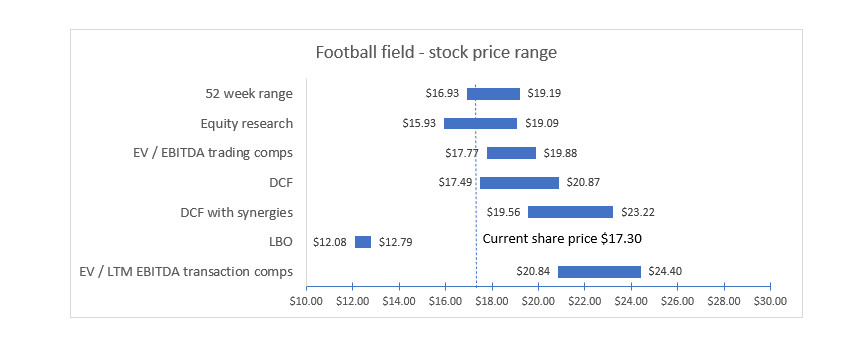
Below are the stock price ranges that we shall be building the football field for and the associated valuation methodologies. Arrange the valuation data as a table in Excel. The example below shows share prices, but it can be used to display Enterprise values or any other valuation measurement.

You can copy and paste this table into Excel to use as an example. Ensure your table does not include any blank rows (if it does, delete them).
Method 1: using a clustered bar chart
(Please scroll down for Method 2 – using a “difference” column and a stacked bar chart.)
2. Method 1 – Create a clustered bar chart
Select the entire table (including headers), then select the “Insert” menu from the ribbon, and click on the little diagonal arrow at the bottom of the “Charts” group (Keyboard shortcut ALT N, K). If you are using your mouse, refer to the circled options in the image below for where to click.

In the charts menu, select “All charts”, “Bar” and then the “Clustered Bar” and hit OK, as shown below:

Now you should have a clustered bar chart.

A legend will appear, either to the side of the chart or under the chart, as circled above.
The legend must be deleted: click on it and hit the delete key. You may also want to include an appropriate title for your chart, or delete it (by clicking on it and hitting the delete key) as necessary. I have added a title “Football field – stock price range”.
3. Method 1 – Format the data series
Right-click on longer bars (orange in the image), which will select all of the bars of the same color and select “Format Data Series”, which will open the related menu as a right panel to your excel sheet.

Under “Series options”, change the “Series overlap” to 100%, as shown below:

The two series should now overlap, so the chart shows only one bar for each valuation method, as in the image below:

4. Method 1 – Stack the series
Right-click on any bar to select the series and choose “Select data”. Select “Min” and move it down by clicking on the down arrow, as shown below:

Your chart should look like this:

5. Method 1 – Hide the series
Right-click on one of the long bars (the blue bars in our example) to select the series and choose “Format Data Series”. Click on “Fill” and choose the color as “White” (to match the chart background), as shown below. Do the same with the “outline” too:

This has hidden the series, so your chart should show floating bars for each valuation methodology as below:

6. Method 1 – Add data labels
Click on the series colored white and from the ribbon above select “Chart design”, followed by “Add chart element”, then “Data labels” and then “Inside end” (Keyboard shortcut after selecting the white series – ALT JC, A, D, E). Alternately, you can also Right-click on the series twice to bring the data labels and then format them to inside end by select “Format Data Labels”, then choose “Inside End” for label position.

Now right-click on the floating bar (the orange bars in the chart above) and select “Add Data Labels”. At this stage your chart should look like this:

7. Method 1 – Adjust the formatting
Remove the vertical gridlines by clicking on them and hitting the delete key. Right-click on the X Axis labels and select “Format Axis”. Change the parameters to adjust the value range and to make any other formatting changes as required (for example, to change the font or the number of decimals). An example is shown below – I have changed the minimum range to 10.00:

You may also want to expand the chart to the right, to stretch the valuation ranges. At this stage, your chart should look like this:

8. Common for Method 1 & 2 – Add a vertical line for the current market price
Click on the “Insert” menu, select “Shapes” and then select the Line. Draw a vertical line on the chart, positioning it where relevant.

If necessary, you can change the line formatting (for example, to have a dashed line or to change its color) by right-clicking the line and selecting Format Shape or from the ribbon menu “Shape format”, followed by “Shape outline”, then “Dashes” and selecting the option you prefer.

You may also want to add a text box to the chart (“Insert” menu, “Text box” or keyboard shortcut ALT N, ZT, X) to show the current value and add the relevant data to the text box – like in my case I have added “Current share price $17.30”.
If you’d like to show the currency, right click on the numbers and select “Format data labels”. In the right panel, select the label options (green chart), then “Number” and adjust the category to “Currency” and choose the appropriate symbol for your currency – I have chosen $ below and 2 decimal places.

You may also change the color of the bar chart matching your standard colors by right clicking on the series and choosing the appropriate fill color option. In my case, I have changed the final color of the floating bars to blue.
9. Finished
Congratulations! Your football field chart is now ready to be used. This is what mine looks like after all the steps followed above:

Method 2: using a stacked bar chart
2. Method 2 – Difference
Add a column between Min and Max values – keeping your cursor in the Max column, hit keyboard shortcut “ALT H I C”. Label it “difference” and calculate the difference by subtracting the “Min” value from each of the “Max” values, as shown below:

3. Method 2 – Insert chart
Select the entire table and insert a stacked bar chart – keyboard shortcuts – CTRL A inside the table followed by ALT N, K and choose the stacked bar chart as shown below:

You should get a chart as below:

A legend will appear, either to the side of the chart or under the chart, as circled above.
The legend must be deleted: click on it and hit the delete key. You may also want to include an appropriate title for your chart, or delete it as necessary. I have added a title “Football field – stock price range”.
3. Method 2 – Add the data labels
Click on the “Min range” – the blue bars and from the ribbon above select “Chart design”, followed by “Add chart element”, then “Data labels” and then “Inside end” (Keyboard shortcut after selecting the blue series – ALT JC, A, D, E). Alternately, you can also Right-click on the series twice to bring the data labels and then format them to inside end by select “Format Data Labels”, then choose “Inside End” for label position.

Now select the “Max range” – the grey bars and do the same thing, except select the data labels to be at the “Inside base”. Now your chart should look like below:

4. Method 2 – Hide the series
Now we need to hide all the blue bars and the grey bars so we are going to select them and choose “Fill” color option as “No Fill” as shown below:

Repeat the steps for “Outline” (it sits right next to “Fill” in the image above) and select “No outline”.
Now repeat both the steps for the Grey bars (Max range). Your chart will look as shown below:

5. Method 2 – Adjust the X Axis
Click on the X axis and adjust the axis bounds between 10 and 30 for a more legible chart.

You may want to stretch your chart by dragging the right edge of the chart to an appropriate width and your chart will look like below:

Now you may follow from Step 8 of Method 1 for formatting the data labels and adding a vertical line for the current share price as well as other formatting options.
Here’s what my final chart looks like with Method 2:

Voila, Now you know 2 methods to create a football field chart.
Happy charting!
Knowledgebank published by Rasna Saini