

Microsoft released its new version of Excel at the end of January 2013. None of the new features are mind blowing from a financial modeling perspective. However, analyzing data, charting and pivot tables are now more user friendly. There are also a few time-saving new functions, and you will notice some tweaks to the look and feel of the working environment.
Excel 2013 integrates nicely with the Microsoft version of cloud storage called SkyDrive. After setting up a Microsoft account, you can use SkyDrive to store and share Office 2013 documents. You can even upload your favorite financial model to Facebook! However, we do not expect organizations to adopt SkyDrive, primarily for security reasons. Below we review the new features in Excel 2013, listed in order of relevance for financial analysis and modeling.
New Functions
Excel 2013 has forty-eight new functions that were not available in previous versions of Excel. Not all of these functions are applicable to financial modeling purposes. My favorite ones are:
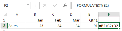
- FORMULATEXT – Returns a formula as a string
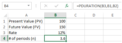
- PDURATION – Solves for n in the following financial math formula FV = PV * (1+r)n
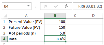
- RRI Solves for r in the following financial math formula FV = PV * (1+r)n
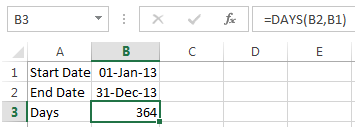
- DAYS Return the numbers of days between two dates
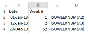
- ISOWEEKNUM Returns the ISO week number of the year for a given date
Flash Fill
Flash Fill is a time-saving feature that reads patterns in adjacent columns and automatically fills the remaining cells in a column based on those patterns. It is useful when you need to concatenate cells or separate information in cells without wanting to write a cumbersome formula.
- Example – Splitting input data
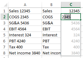
The worksheet below shows data downloaded from an external source. Separating the heading from the value can now be done very quickly using Flash Fill.
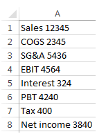
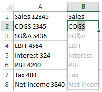
In cell B1, you would input the line item heading corresponding to the cell to the left (in this example type Sales). In cell B2, as you start typing the next line item heading (COGS), you will see Excel automatically filling the remaining rows underneath, as shown below. On pressing enter, Excel will fill the whole column.
Using the same logic, Flash Fill can also be used to extract automatically the numbers from column A, as shown below.
- Example – Concatenating Data
Flash Fill can be used to concatenate cells. The worksheet below shows a list of employees.
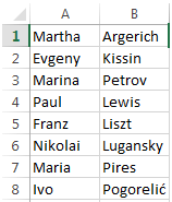
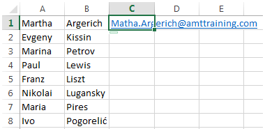
Let us assume that our task is to input each employee’s email address in the worksheet. In cell C1, we write the email address for Martha, as shown below.
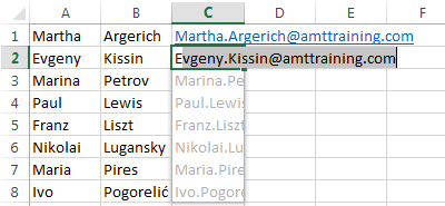
As you start writing the email address for the next employee (Evgeny), Flash Fill will pick up the pattern and will automatically fill the rows underneath.
Quick Analysis Tool
When a user selects a range of data, Excel 2013 shows a box in the bottom right hand corner of the selection containing “Quick Analysis” options. On clicking the box, a number of tools will appear. Alternatively, select the data and press CTRL + Q to show the quick analysis options.
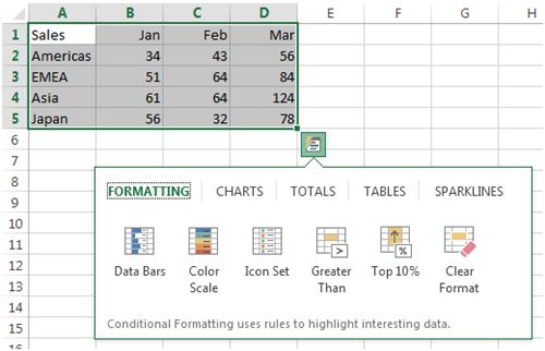
As you hover over the options with the mouse, Excel 2013 shows a live preview of the result. You can use this functionality to quickly add totals to your data, create charts, Sparklines and more. Quick Analysis does not add any new tools to Excel (all the options were already available in previous versions of Excel), it just makes existing tools immediately more accessible.
Recommended Charts
Excel 2013 can recognize patterns in your data and recommend charts that best illustrate those patterns. To use this feature, select the data you wish to chart and choose Recommend Charts on the Insert ribbon.
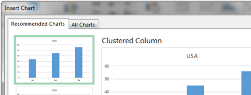
Chart Formatting Control
Formatting charts in Excel 2013 is now easier. When selecting a chart, three new option boxes appear to the right of the chart: chart elements; chart styles; and chart filters.
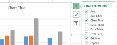
Chart Animation
If you change a data entry in the source table of a chart, you will see the chart change in an animated way. For example, suppose you change a number in a source table for a bar chart from 10 to 100, you will see the bar in the chart corresponding to the data point gradually increase from 10 to 100.
Recommend PivotTables
Recommend PivotTables will suggest a pivot table that is most suitable for the source data. To use this tool, click any cell within the source data and choose Recommend PivotTables from the Insert Ribbon.
Timeline Filter for PivotCharts or PivotTables
Timeline Filter allows you to easily filter data in a PivotTable or PivotChart over a range of dates. For example, the Timeline Filter is being used to filter the PivotTable below to show total sales for January and February only.
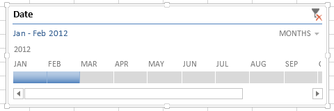
To activate the Timeline Filter, create a PivotTable based on data that includes dates. Select the PivotTable and then choose Insert Timeline from the Analyze Ribbon (the analyze ribbon will only appear when the PivotTable is selected).
To increase or decrease the time period, click and drag the start or end points of the timeline with the mouse. To change the time period, click the period menu in the top right hand corner of the Timeline and choose from: Years; Quarters; Months; or Days.
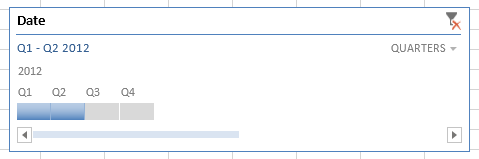
The PivotTable above now shows sales data for Q1 and Q2.
What is missing?
I was disappointed to find no new significant keyboard shortcuts in Excel 2013. I was expecting Microsoft to introduce new shortcuts similar to the ones provided by our free Excel add-in, which we will be updating later in the year to ensure compatibility with Excel 2013. Also the format styles functionality has not been updated since the 2007 version. It is still very cumbersome, even worse than in Excel 2003. I would have liked to see a style manager in Excel 2013 that allows deleting multiple styles at the same time (a feature that is available in the AMT add-in). Selecting font and cell colors from the color palette is still not as streamlined as it used to be in Excel 2003. Selecting colors from the palette using keyboard shortcuts is still unnecessarily time intensive.
What do you think?
Are you using Excel 2013 yet? Let us know how you feel about the new version and any features you are looking forward to.
Please do not hesitate to contact us, if you are having trouble viewing or accessing this article.
Copyright© 2016 AMT Training