

Discover some of the most useful lesser known features that can have a huge impact on your financial modeling workflow when using Microsoft Excel.
Excel camera tool
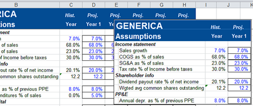
This feature enables you to make dynamic photos of the Excel screen. This means that the photo will update as the captured information in the worksheet updates. This tool is very useful to see how other parts of a model are impacted when the assumptions change.
To install this feature:
- Right click the quick access toolbar and choose “Customize Quick Access Toolbar”. The Excel Options dialog box will open.
- Choose “All Commands” from the “Choose from commands” dropdown
- Scroll down the list of commands until you find the “Camera” feature
- Choose the “Add” button to install the camera function on the quick access toolbar
- Choose “OK” to close the Excel Options dialog box
To use this feature:
- Select an area of the screen to capture
- Click the Camera button on the quick access toolbar
- Click a destination point on the screen for the dynamic picture. The picture will appear as an object on the Excel worksheet. As you change the data captured in step 1 above, you should see the picture update.
Be careful: don’t use this feature as an infinite resource. The dynamic pictures consume memory and should ideally be deleted once you have used them.
Excel watch window
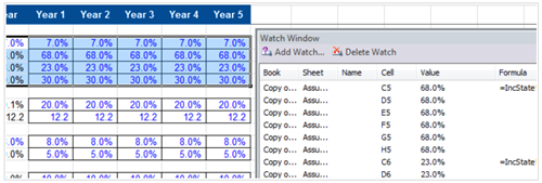
A great feature that allows you to see the content of specified cells from a completely different part of the model. Similar to the Camera tool, this feature is very useful when you want to see how changing assumptions impact different parts of the model.
To use this feature:
- Select the cell or cells to “watch”
- Click the “Watch Window” button from the formulas ribbon. The Watch Window dialog box will appear
- Click the “Add” button and confirm by clicking OK from the “Add Watch” dialog box
The “Watch Window” will now display the cell or cells being watched, their values and formulas contained within them.
Excel speech
Yes you can have Excel speak the content of cells to you! Useful if you are feeling lonely at your desk late one evening! Joking aside, this feature probably sounds very gimmicky, but it’s actually a useful tool when you are trying to reconcile numbers in your models.
To install this feature:
- Right click the quick access toolbar and choose “Customize Quick Access Toolbar”. The Excel Options dialog box will open
- Choose “All Commands” from the “Choose from commands” dropdown
- Scroll down the list of commands until you find the “Speak Cells” feature
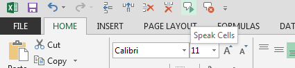
- Choose the “Add” button to install the speak cells function on the quick access toolbar. Consider also adding the Stop Speaking Cells option
- Choose “OK” to close the Excel Options dialog box
To use this feature:
- Enter a sentence or a number into cell or a range of cells
- Select the cell or range of cells
- Click the “Speak Cells” button on the Quick Access Toolbar. Excel will speak the content of the cell or cells back to you!
Tip
make sure the volume on your computer is high enough to hear Excel speak. You may also need to wear headphones, depending on your set up.
If the data you want Excel to speak back at you is in a two dimensional range, you can use the “Speak Cells by Column” or “Speak Cells by Row” options to specify the order. Furthermore, you can also activate the “Speak Cells on Enter” feature, to have Excel speak the content of a cell back at you after pressing enter. Run through the first 5 steps above to install these features on the Quick Access Toolbar.
Sparklines in Excel
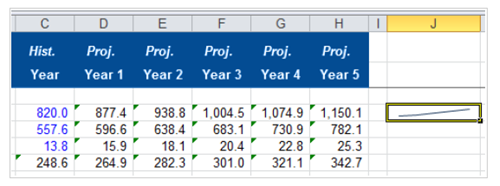
These are mini charts that appear within a cell. However this cool feature is only available from Excel 2010 onwards. This feature is useful if you want to graphically represent the progression of a forecast in your model.
To use this feature:
- Select the cell to contain the spark line
- Go the “Insert” ribbon and choose “Line” from the “Sparklines” group. The Create Sparklines dialog box will appear
- Select the source data for the spark line using the mouse. The range you select will appear in the Data Range edit box
- Choose OK. A mini chart (aka Sparkline) will appear in the chosen cell
Once you are familiar with using the “Line” feature, run through these steps again and try “Columns” and “Win / loss” mini charts too!
Please do not hesitate to contact us, if you are having trouble viewing or accessing this article.
Copyright© 2016 AMT Training