

Did you think that conditional formatting for constants (blue font color for example) was impossible? Well think again!
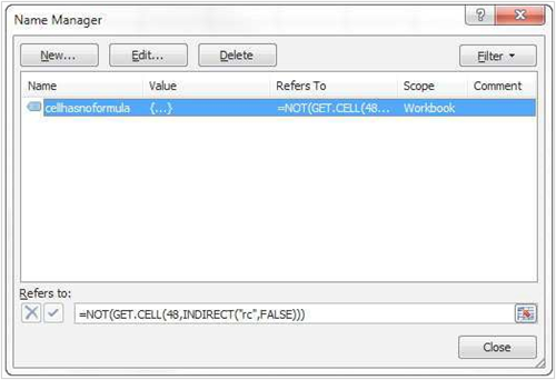
Create a new named range called cell has no formula. In the ‘Refers to:’ box type the following: =NOT(GET.CELL(48,INDIRECT(“rc”,FALSE)))
How to create a new conditional formatting rule
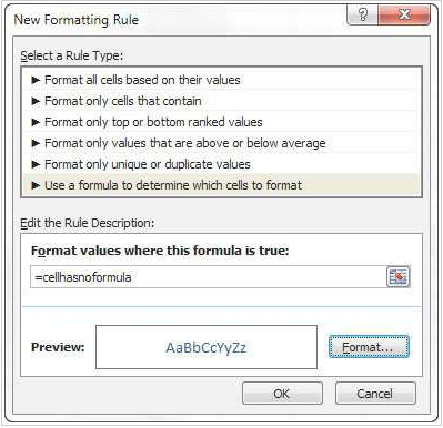
Select some cells (preferably with both formulas and constants in) to apply your conditional formatting to create a new conditional formatting rule, choose the ‘use a formula…’ option. Type the following formula in the ‘rule description’: =cellhasnoformula
How to create conditional formatting for constants
Click the format button and choose the formatting you would like for your constants (blue font color for example). Click OK twice to apply the formatting. The cool thing about this is, that if any cell in the range changes from being a constant to a formula (or vice versa), the font colour will automatically change!
Please do not hesitate to contact us, if you are having trouble viewing or accessing this article.
Copyright© 2016 AMT Training