

Quicker keyboard shortcuts
In Excel 2007, the ALT keyboard shortcuts were very slow. For example, if you pressed the keyboard shortcut sequence ALT+E+S+T too quickly (or the same speed as Excel 2003), Excel 2007 would simply not register the shortcut and therefore not run the command. Keyboard shortcut veterans found this really frustrating as this would slow down the modeling process! One of the major improvements in Excel 2010 is that this problem has been removed! You can now press ALT keyboard shortcuts at normal speed.
Customizing the ribbon
In Excel 2010, you can customize the ribbon, which is great news for modelers! You can now set up a perfect ribbon with a set of commands applicable for financial modeling purposes. You can create custom ribbon tabs and groups and rename or change the order of the built-in tabs and groups.
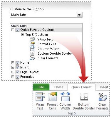
To customise the ribbon, right-click on an existing ribbon tab, choose customise the ribbon from the menu. The options in the Customize Ribbon dialog box are fairly self explanatory. You can also share your customisations with colleagues: to export your customisations, use the Import/Export button at the bottom of either the Customize Ribbon or Quick Access Toolbar pane of the Excel Options dialog box. This creates a file which you can email to a colleague. Your colleague can then import the file using the same Import/Export button.
The office icon button has been replaced by a file menu
In Excel 2007, Microsoft introduced the Office Icon button, which gave you access to most of the commands in the old File menu. In Excel 2010, Microsoft has reverted back to the File menu. However, this new File menu gives you access to something called “Backstage View”.
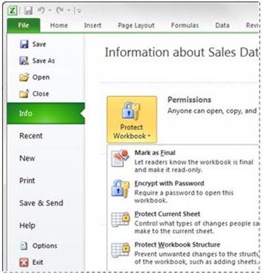
When you open the File menu, Excel now fills 100% of your screen with a three panel backstage view. You can use this view to create new files, open existing files, save, send, protect, preview, and print files, set options for Excel, and more. The first panel works like a navigation bar, the second panel contains a variety of commands related to the choice from the first panel and the third panel provides a view of the additional settings related to the commands chosen in the second panel. Useful keyboard shortcuts are as follows:
|
Keyboard shortcut |
Description |
|
ALT+F+S(or CTRL+S) |
Save |
|
ALT+F+A (or F12) |
Save As |
|
ALT+F+O (or CTRL+O) |
Open |
|
ALT+F+C (or CTRL+F4) |
Close current document |
|
ALT +F+X (or ALT+F4) |
Exit Excel |
The proper way to close backstage view is to press the Esc key or click any other ribbon with the mouse.
Sparklines
Sparklines are tiny charts that fit in a cell. They enable you to visually summarize trends alongside data. Because sparklines show trends in a small amount of space, they are especially useful where you need to show a snapshot of data in an easy-to-understand visual format. In the following image, F2 contains a column sparkline and F3 contains a line sparkline.
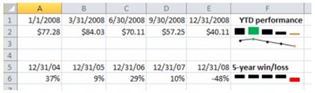
A sparkline in cell F6 shows the 5-year performance for the same stock, but displays a Win/Loss bar chart that shows only whether the year had a gain or a loss. To create a sparkline:
- Select an empty cell or group of empty cells in which you want to insert one or more sparklines.
- On the Insert tab, in the Sparklines group, click the type of sparkline that you want to create: Line, Column, or Win/Loss
- In the Data box, type the range of the cells that contain the data on which you want to base the sparklines.
Faster ways to paste special
Excel 2007 introduced the cool CTRL + ALT + V shortcut to activate the paste special dialog box, which I liked so much that I believe it is worthy of mention in this technical update! Excel 2010 introduces another way to paste special. When you do a normal copy and paste, a little clipboard appears on your worksheet which you can open by pressing CTRL. If, for example, you then hover over the paste values icon on this clipboard, you will learn that V is the relevant shortcut. So now you could press the following keyboard sequence to copy and paste values:
|
CTRL+C |
Copy |
|
CTRL+V |
Paste |
|
CTRL |
to open the Paste Options dialog |
|
V |
to change the paste to values |
Recover previous saved versions
If you accidentally close a file without saving it, it is now much easier for you to recover the last Autosaved version of the file. To find the unsaved version, open the File menu and choose Recent and specify the autosaved file to open. However, this new feature is no compensation to manually saving files with CTRL + S. You should continue to save file manually to minimise the risk of losing your work. You can also roll back to the previous autosaved version of a file by opening the File menu and choosing Info and then Manage Versions.
|
Note You must set the “Save AutoRecover information every x minutes” and “Keep the last autosaved version if I close without saving” options in the Excel Options for these features to work. |
Protected view
Excel 2010 includes a protected view which allows you to make more informed decisions before exposing your computer to viruses. Any file that comes from a potentially dangerous location is open in the new Protected view. In this view, you can look through the file and even take a look at the VBA code of macros without exposing your computer to vulnerabilities. If you establish that the file is safe, you can click a button to convert the file to regular mode.
Trusted documents
The trusted documents feature is designed to make it easier to open workbooks and other documents that contain active content, such as macros or data connections. Now, after you confirm that active content in a workbook is safe to enable, you don’t have to repeat yourself. Excel 2010 remembers the workbooks you trust so that you can avoid being prompted each time you open the workbook.
Improved charting
There are three key charting improvements in Excel 2010. These are:
|
New charting limits |
The limitation on the number of data points that can be created on a chart has been removed. The number of data points is limited only by available memory. This enables people to more effectively visualize and analyze large sets of data. |
|
Quick access to formatting options |
You can instantly access formatting options by double-clicking a chart element. |
|
Macro recording for chart elements |
Recording a macro while formatting a chart or other object did not produce any macro code. In Excel 2010, however, you can use the macro recorder to record formatting changes to charts and other objects. |
Improved conditional formatting
Conditional formatting makes it easy to highlight interesting cells or ranges of cells, emphasize unusual values, and visualize data by using data bars, color scales, and icon sets. Excel 2010 includes even greater formatting flexibility:
- New icon sets
Icon sets, introduced in Office Excel 2007, let you display icons for different categories of data, based on whatever threshold you determine. For example, you can use a green up arrow to represent higher values, a yellow sideways arrow to represent middle values, and a red down arrow to represent lower values. In Excel 2010, you have access to more icon sets, including triangles, stars, and boxes. You can also mix and match icons from different sets and more easily hide icons from view—for example, you might choose to show icons only for high profit values and omit them for middle and lower values.
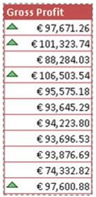
- More options for data bars
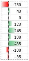
Excel 2010 comes with new formatting options for data bars. You can apply solid fills or borders to the data bar, or set the bar direction from right-to-left instead of left-to-right. In addition, data bars for negative values appear on the opposite side of an axis from positive values, as shown here:
- Other improvements
When specifying criteria for conditional or data validation rules, it’s now possible to refer to values in other worksheets in your workbook.
Improved filtering
Excel 2010 includes some very cool filtering enhancements. These are as follows:
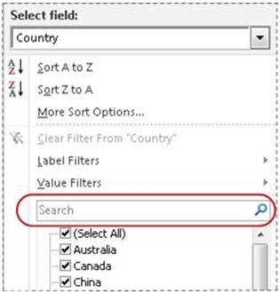
- New search filter
When you filter data in Excel tables, PivotTables, and PivotCharts, you can use a new search box, which helps you to find what you need in long lists. For example, to find a specific company in a list that contains over 100,000 businesses, start by typing your search term, and relevant items instantly appear in the list. You can narrow the results further by deselecting the items you don’t want to see.
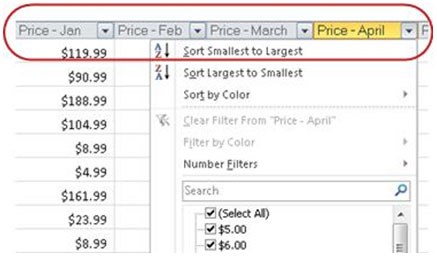
- Filter and sort regardless of location
In an Excel table, table headers replace regular worksheet headers at the top of columns when you scroll down in a long table. AutoFilter buttons now remain visible along with table headers in your table columns, so you can sort and filter data quickly without having to scroll all the way back up to the top of the table.
Please do not hesitate to contact us, if you are having trouble viewing or accessing this article.
Copyright© 2016 AMT Training