
Note on Compatibility: Before we begin, we’d like you to know that this function is currently available to Office 365 subscribers in the Monthly channel. It will be available to Office 365 subscribers in the Semi-Annual channel starting in July 2020.
If you have ever found Vlookup confusing and have had to read about the function arguments… then you will like Xlookup. If you have liked working with Vlookup, you will love Xlookup even more.
Xlookup is an awesome function and we cannot wait to use it in our classes! Xlookup can be used to replace several Excel functions such as Vlookup (and Hlookup), Index with a nested match, and others.
How is Xlookup different from Vlookup?
- Unlike Vlookup, which uses a single array followed by a column index number, Xlookup uses separate lookup and return arrays, which allows you to look in one column for a search term, and return a result from the same row in different column
- Vlookup requires the lookup column to be the 1st column in the array, but Xlookup does not have this restriction, so you can use any column as your lookup column.
- The lookup array and return array are separated, so they can be anywhere on the sheet or workbook!
- The return array replaces the column index number in Vlookup. This means that you can happily add or remove columns from your table, without impacting the output of Xlookup.
- Xlookup by default gives you an exact match. That means that you do not need to sort your data prior to the search
- Vlookup required either a sorted list in the 1st column of the array, or a specific FALSE argument at the end of the function
- Xlookup also allows you to search for the “next smaller” or the “next larger” item of the lookup value
- Xlookup even allows you to search with a wildcard match when you know only some part of the lookup value
- Xlookup allows you to search for your item from top to bottom (or left to right) as well as from bottom to top (or right to left) by specifying a dedicated argument
- Xlookup allows you to specify a if_not_found argument in order to deal with errors. This means that there is no need to use a IFERROR function to manage errors.
- Xlookup is able to return an array of outputs using a single formula! This behavior is called spilling, because it spills the set of output values into the neighbouring cells
- With Vlookup, you had to copy the formula over a range of cells
- Vlookup uses an entire table array and hence also uses more computing power. Xlookup needs to handle only lookup and return arrays hence uses less computing power
Function arguments
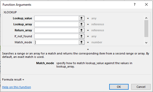
Here is how you write it:
= Xlookup(lookup_value,lookup_array,return _array,[match_mode],[search_mode],[if_not_found])
The first 3 arguments are required and the next 3 are optional.
Examples:
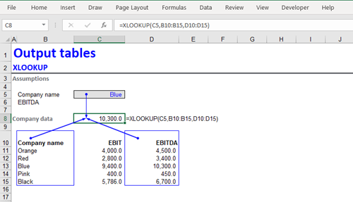
- Let’s start with a basic Xlookup using only the required arguments.
In the image below, the Xlookup function is in cell C8 – notice that there is no sorting of the lookup array and there is no column index number – just the return array, and there is no final argument (true/false) stipulating a approximate/exact match. The Xlookup formula set up is clearly more intuitive than Vlookup.
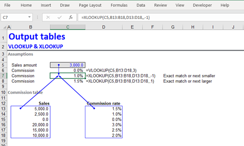
- Now let’s do an approximate match.
In the example below, we want to find the commission rate for a sales amount of 3,000.
The spreadsheet image shows the results of: a) Vlookup, b) Xlookup with an exact match or smaller and c) Xlookup with an exact match or larger.
Notice that the lookup array is not sorted, therefore Vlookup does not work! Vlookup would work only if the lookup values were provided as a sorted list. On the other hand, Xlookup works just fine, even though the lookup values are not sorted!
Notice also that we can choose a ‘next smaller’ or ‘next larger’ method, to decide which output value should be chosen. - Let’s now look at Xlookup with its spilling behavior
We wrote the Xlookup function in cell D11. Notice the function arguments:- The lookup value and the lookup array are relative references
- The return array is 2 dimensional (a table).
Once the formula has been written in D11, when you press Enter the formula ‘spills’ over onto the cells on the right (D11:H11), without the need to copy&paste it. There are no formulas in cells E11:H11!
Hopefully, we have convinced you that Xlookup is superior to the ‘old’ Vlookup function! If you use Xlookup, you will no longer need to nest match functions inside Vlookup and you can even use Xlookup to replace Index and other Excel functions.
Happy exploring!